Script
library("sf")
library("terra")
library("lidR")
library("raster")
library("dbscan")
library("tidyverse")
library("leaflet")
library("RColorBrewer")
library("rgl")
library("knitr")Understanding forest structure and characteristics in Letchworth Learning Forest
Tina Ni
December 7, 2024
Forest structure plays a critical role in understanding forest biodiversity and ecosystem services (MacKinnon, 2012; Wang et al., 2024). However, measuring forest structure through traditional field data collection is challenging due to time and funding constraints, particularly in large forests. The introduction of remote sensing has been a key driver in obtaining large forest structure data indirectly, while lessening the burden of time and funding limitations (Wulder et al., 2012). In this project, I utilized publicly available remote sensing data to answer a few questions about the Letchworth Teaching Forest’s structure and assessed the effectiveness of remote sensing as a stand-alone method for forest structure analysis.
These questions include:
1. What is the approximate tree population?
2. Where are the locations of individual trees?
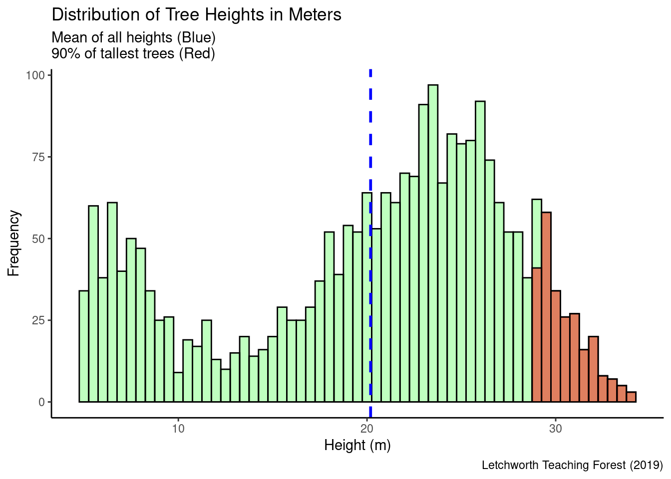
3. What is the distribution of tree heights in the study site?
4. Where are the 90% percentile of tallest trees located?
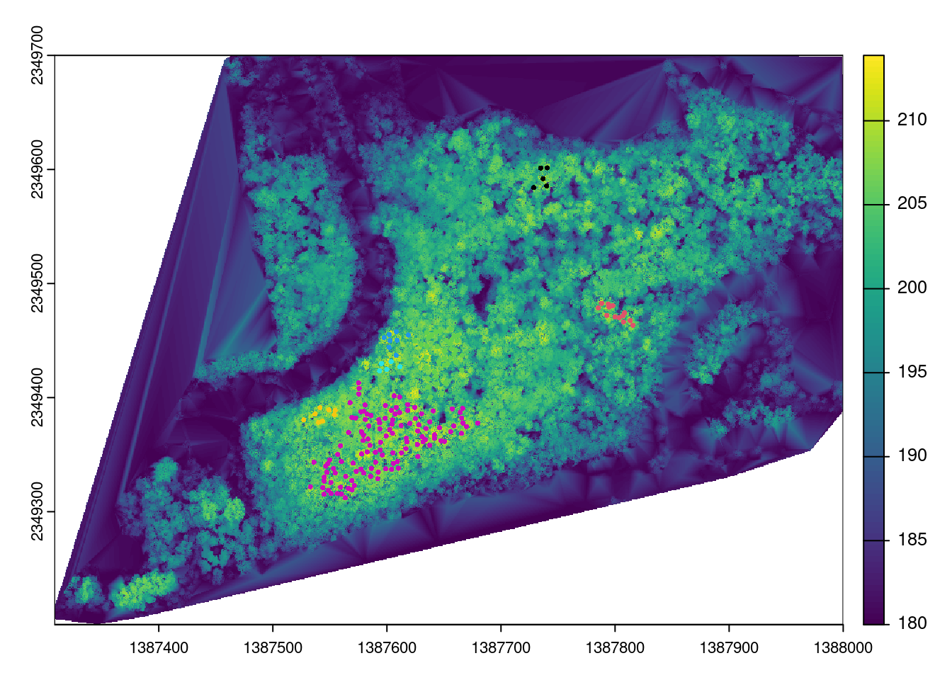
5. Is there spatial clustering of tall trees?
This project utilized the most recent (2019) LiDAR point cloud data (USGS Lidar Point Cloud NY_3County_2019_A19 E1387n2349_2019 - ScienceBase-Catalog, n.d.) to assess vertical forest structure within the Letchworth Learning Forest near the Ellicott Complex. The LiDAR data, originally projected horizontally in NAD83 (2011) and vertically measured in meters, was processed to answer question listed above. Using the lidR and dbscan packages, Z-values from the point-cloud data were filtered and analyzed to identify individual trees, calculate tree heights, and determine spatial clustering of the tallest trees within the study area. The resulting dataset, named filterOUT_las, was re-projected into WGS84, enabling tree locations and clustering pattern visualization on an interactive Leaflet map.
Critical R packages utilized in this project included:
Below is the R script:
polygon_coords <- matrix(c(
  1388000, 2349355, #right bottom corner
  1388000, 2349700, #right top corner
  1387450, 2349700, #mid top corner
  1387450, 2349450, #mid mid corner
  1387300, 2349200, #left bottom corner
  1387350, 2349200, #mid bottom corner
  1388000, 2349355  #right bottom corner
), ncol = 2, byrow = TRUE)

## Bounding Box has been given CRS associated with las-CRS
polygon_sf <- st_sfc(st_polygon(list(polygon_coords)), crs = st_crs(las))## Reproject the las to 4326 for Leaflet
options(digits = 15)
las84 <- st_as_sf(las_clipped, coords = c("X", "Y"), crs = 26918) # crs was NAD83(2011)
las84 <- st_transform(las_clipped, crs = 4326)
## Create a dataframe of points lat and long to check if st_transform worked
las_df <- data.frame(lat = st_coordinates(las84)[, 2],
long = st_coordinates(las84)[, 1])
unique(las_df$lat)[1] 43.005 43.006 43.007 43.009 43.008 [1] -78.797 -78.796 -78.795 -78.794 -78.793 -78.792 -78.791 -78.790 -78.789
[10] -78.788 -78.787## LidR functions to find individual trees
chm <- rasterize_canopy(filterOUT_las, 0.25, pitfree(subcircle = 1))
tree_tops <- locate_trees(chm, lmf (ws=5))
filtered_tree_tops <- tree_tops %>%
filter(Z >= 190)
#plot(chm, col = height.colors(50))
#plot(sf::st_geometry(filtered_tree_tops), pch = 3)
#plot(sf::st_geometry(filtered_tree_tops), add = TRUE, pch = 3)
nintypercent <- quantile(filtered_tree_tops$Z, 0.90)
tall_trees <- filtered_tree_tops[filtered_tree_tops$Z > nintypercent,]
coords <- st_coordinates(tall_trees)tree_Z <- as.data.frame(filtered_tree_tops$Z)
colnames(tree_Z) <- c("height")
ind_trees <- tree_Z$height - 190
ind_trees <- as.data.frame(ind_trees)
tall_trees_height <- as.data.frame(tall_trees$Z - 190)
colnames(tall_trees_height) <- c("height")
## in meters
mean <- mean(ind_trees$ind_trees)
mean <- round(mean, 2)
subtitle = paste("Total trees = ", nrow(ind_trees), " trees \nMean (Blue) = ", mean,"\n90% of tallest trees (Red)")
ggplot()+
geom_histogram(data = ind_trees, aes(x = ind_trees), binwidth = 0.5,, color = "black", fill="green", alpha = 0.25)+
geom_histogram(data = tall_trees_height, aes(x = height), binwidth = 0.5,, color = "black", fill="red", alpha = .5)+
geom_vline(aes(xintercept = mean(ind_trees$ind_trees)), color="blue", linetype="dashed", linewidth=1)+
theme_classic()+
labs(title = "Distribution of Tree Heights in Meters", x = "Height (m)", y = "Frequency",
subtitle = subtitle,
caption = "Letchworth Teaching Forest (2019)")
| Tree ID | Height (m) | Location |
|---|---|---|
| 1 | 3.7 | POINT Z (1387490.125 234969… |
| 2 | 2.8 | POINT Z (1387494.875 234969… |
| 3 | 5.6 | POINT Z (1387469.125 234969… |
| 4 | 2 | POINT Z (1387848.125 234969… |
| 5 | 8.7 | POINT Z (1387464.625 234969… |
| 6 | 3.3 | POINT Z (1387470.625 234969… |
| 7 | 6.5 | POINT Z (1387469.875 234968… |
| 8 | 1.8 | POINT Z (1387479.375 234967… |
| 9 | 3.1 | POINT Z (1387861.375 234967… |
| 10 | 2 | POINT Z (1387476.625 234967… |
| Tree ID | Height (m) | Location | |
|---|---|---|---|
| 223 | 223 | 19.71 | POINT Z (1387784.125 234960… |
| 240 | 240 | 19.88 | POINT Z (1387740.375 234960… |
| 243 | 243 | 19.76 | POINT Z (1387734.875 234960… |
| 256 | 256 | 19.86 | POINT Z (1387785.375 234959… |
| 307 | 307 | 21.54 | POINT Z (1387736.875 234959… |
| 354 | 354 | 19.87 | POINT Z (1387740.125 234958… |
| 366 | 366 | 19.46 | POINT Z (1387728.625 234958… |
| 387 | 387 | 20.69 | POINT Z (1387846.875 234958… |
| 452 | 452 | 19.55 | POINT Z (1387777.625 234957… |
| 505 | 505 | 19.68 | POINT Z (1387739.125 234956… |
knitr::opts_chunk$set(global.device = TRUE)

dbscan_result <- dbscan(coords, eps = 12, minPts = 5)

tall_trees$dbscan_cluster <- as.factor(dbscan_result$cluster)
colorsize = length (unique (tall_trees$dbscan_cluster))


## Filter out first cluster
cluster <- tall_trees %>%
filter(dbscan_cluster != 0)
plot(chm)
plot(cluster[3], pch = 16, cex = .5, col = factor(cluster$dbscan_cluster), main = "Tree Clusters", add = TRUE)
pal <- colorFactor(brewer.pal(4, "Set1"), domain = tall_trees$dbscan_cluster)

st_tall_trees <- st_transform(tall_trees, crs = 4326)

st_tall_trees_filtered <- st_tall_trees %>%
  filter(dbscan_cluster != 0)
st_tall_trees_filtered$Z <- st_tall_trees_filtered$Z - 180


leaflet (st_tall_trees_filtered) %>%
  setView(lng = -78.793, lat = 43.007, zoom = 15)  %>%
  addTiles() %>%
  addCircleMarkers(
    radius = 2,
    color = ~pal(dbscan_cluster),
popup = ~paste("Tree ID:", treeID, "<br> Height (m):", Z,"<br> Coordinates:", geometry))This study demonstrates the potential of using remote sensing data to assess forest structure with promising results. The analysis indicates a total of approximately 2,018 trees, with individual tree locations identified. Spatial clustering of the tallest trees were observed in six areas. The overall average height across the entire tree population was found to be 13.02 meters. It is important to note that the results , derived solely from remote sensing data and computational analysis, offer only a rough estimate of forest structure characteristics. For more precise and reliable conclusions, incorporating field data is essential to provide a reference for validating the remote sensing analysis.
In conclusion, while remote sensing provides a faster method for assessing forest characteristics, the inclusion of field data is crucial to ensure the accuracy and reliability of the results. Combining both approaches will offer a more comprehensive understanding of forest dynamics.
MacKinnon, A. (2012). Forest Structure: A Key to the Ecosystem. https://www.semanticscholar.org/paper/Forest-Structure-%3A-A-Key-to-the-Ecosystem-MacKinnon/57c825a33e087bd8797333885ebf641ed8416377
USGS Lidar Point Cloud NY_3County_2019_A19 e1387n2349_2019—ScienceBase-Catalog. (n.d.). ScienceBase. Retrieved December 5, 2024,https://www.sciencebase.gov/catalog/item/5f6b632982ce38aaa244d224
Wang, M., Baeten, L., Van Coillie, F., Calders, K., Verheyen, K., Ponette, Q., Blondeel, H., Muys, B., Armston, J., & Verbeeck, H. (2024). Tree species identity and interaction determine vertical forest structure in young planted forests measured by terrestrial laser scanning. Forest Ecosystems, 11, 100196. https://doi.org/10.1016/j.fecs.2024.100196
Wulder, M. A., White, J. C., Nelson, R. F., Næsset, E., Ørka, H. O., Coops, N. C., Hilker, T., Bater, C. W., & Gobakken, T. (2012). Lidar sampling for large-area forest characterization: A review. Remote Sensing of Environment, 121, 196–209. https://doi.org/10.1016/j.rse.2012.02.001